Dimension reduction methods – t-SNE

In the previous blog, we have introduced dimension reduction in single-cell RNA-Sequencing (scRNA-Seq) and PCA as one dimension reduction method. We have learned that single cell data are sparse, noisy, and high-dimensional and that dimension reduction is needed to turn the data into something more manageable. In this blog, we will discuss t-SNE.

What is t-SNE

T-distributed stochastic neighbor embedding (T-SNE) is a method that gives us expression values on a cell-wise basis. First introduced by van der Maaten and Hinton in 2008, t-SNE is a probabilistic dimensionality reduction technique.

Some sources said the motivation behind t-SNE stems from the limitations of PCA.

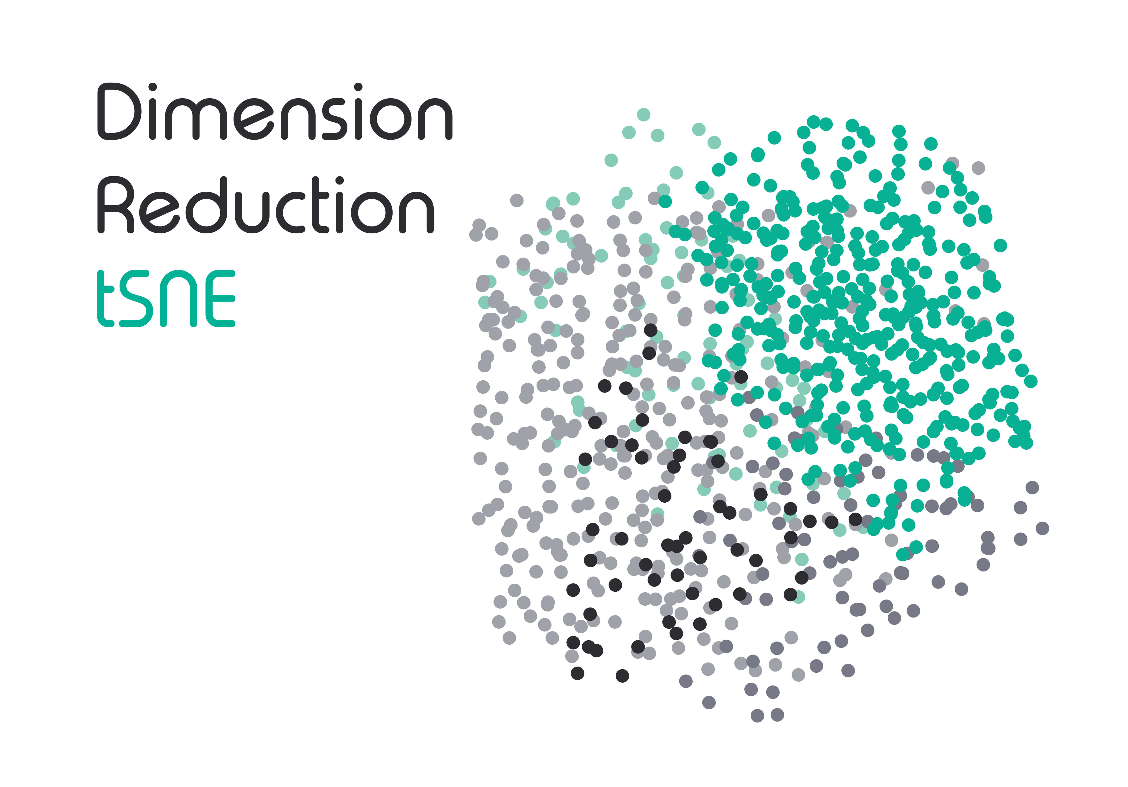
If PCA aimed to maximize global structure and produced some local inconsistencies along the way (far away points end up being neighbors), t-SNE focuses on preserving the local relationships among data points (Fig 1).

PCA is a linear technique while t-SNE is nonlinear and can “unroll” structures more correctly. The algorithm is adaptive to the underlying data, so it carries out different transformations to different regions of data.

T-SNE 101

The math behind t-SNE has 4 equations. The first one sets the symmetry rule, t-SNE calculates the probability of similarity of points in high-dimensional space and then similarly in the corresponding low-dimensional space.
The second equation sets perplexity, which is a parameter that guesses the number of close neighbors each point has. In general, larger datasets mean larger perplexity. By setting perplexity, t-SNE balances the global and local structures of the data. Wattenberg et al. (2016) did an amazing job illustrating this point with multiple simple data sets.

The third one calculates the student’s t-test and the fourth one calculates Kullback-Leibler divergence. The detailed math is explained in the original Maaten paper, but it’s out of scope for our blog today.

Essentially, what these 4 equations do is take a set of points in high-dimensional space and reorganize them as accurately as possible in the lower (typically 2D) dimensions.

T-SNE pros

As a non-linear technique, t-SNE has the amazing ability to work with high-dimensional data. It is user-friendly and often produces more meaningful outputs than many other alternatives.

T-SNE preserves local structure. What this means is that points that are close to one another in the high-dimensional data set will tend to be close to one another in the lower-dimensional chart.

T-SNE is incredibly flexible to different types of input data. It is one recommended choice for scRNA-seq data visualization, for example here or here.

T-SNE cons and how to work with them

Although impressive, the t-SNE outputs are prone to misreading. T-SNE is a dimensionality reduction technique and NOT a clustering technique. T-SNE reduces the number of dimensions and then attempts to find patterns in the data by identifying observed clusters. However, after this process, the input features are no longer the same as they were, and you cannot make any inference based only on the t-SNE output. Cluster size and cluster distance in t-SNE do not have any intrinsic meaning, as illustrated brilliantly by Wattenberg et al. (2016) in this tutorial.

The algorithm of t-SNE means it is good at preserving the local relationships between points but not much of the global data structure.

Running t-SNE multiple times on the same dataset will likely result in different outputs. It’s best to run t-SNE repeatedly to choose the best perplexity parameter, and to average the output. You may also stabilize the overall output through setting a seed to override the random initialization.

Reading t-SNE may require you to pick up on the random noises (“odd” results). This is possible through training and experience. Some of them are addressed and explained clearly by Maaten himself on his website.

T-SNE is computationally heavy. In very large datasets, we need to couple t-SNE with another technique to both (1) increase accuracy and (2) reduce the computational power required. One recommendation suggested coupling of t-SNE with PCA for dense data and TruncatedSVD for sparse data.

Best practices in scRNA-Seq

In scRNA-seq, we often couple t-SNE with PCA. The reason for this is that the mathematical goal of t-SNE is to capture the local relationships between cells (points of a network), whereas PCA will calculate the “true” distance between points in a high dimensional space (we call this the global structure). Using PCA as the first dimensionality reduction technique helps us project our scRNA-seq data into a lower-dimensional subspace. The distances become more real, and t-SNE can display more real relationships between points. Doing so will also reduce computational resources and time needed.

Other best practices that you should also follow include:
(1) Setting the perplexity limit between 5 and 50 (default is often 30)
(2) Run t-SNE repeatedly and average the output

Summary

After the third blog in the series on dimensionality reduction, you now know what t-Stochastic Neighbor Embedding is and how it is used in scRNA-Seq data analysis. In the next blogs, we will continue to discuss the final most popular method of dimensionality reduction: UMAP.

The content of these blogs is only meant to be introductory. If you would like to know more about the mathematical basis or the algorithms of t-SNE, I suggest the following resources:
– The original van der Maaten paper
– T-SNE Python tutorial

If you need scRNA-seq-related help, Dolomite Bio offers end-to-end Single-Cell Consultancy Service that helps you through one or more steps of the workflow:

• Sample preparation
• Library preparation
• Sequencing
• Computational Analysis

Interested queries and/or suggestions for what we should write next in our blog series should be directed to: bioinformatics@dolomite-bio.com

Need help with your single cell data analysis? Check out Dolomite Bio’s new Bioinformatics Service