Dimension reduction methods – UMAP

In the previous blog, we introduced dimension reduction in single cell RNA-Sequencing (scRNA-Seq) as well as PCA and t-SNE dimension reduction methods. We have learned that single cell data are sparse, noisy, and high-dimensional and that dimension reduction is needed to turn the data into something more manageable. In this last blog of the series, we will discuss UMAP.

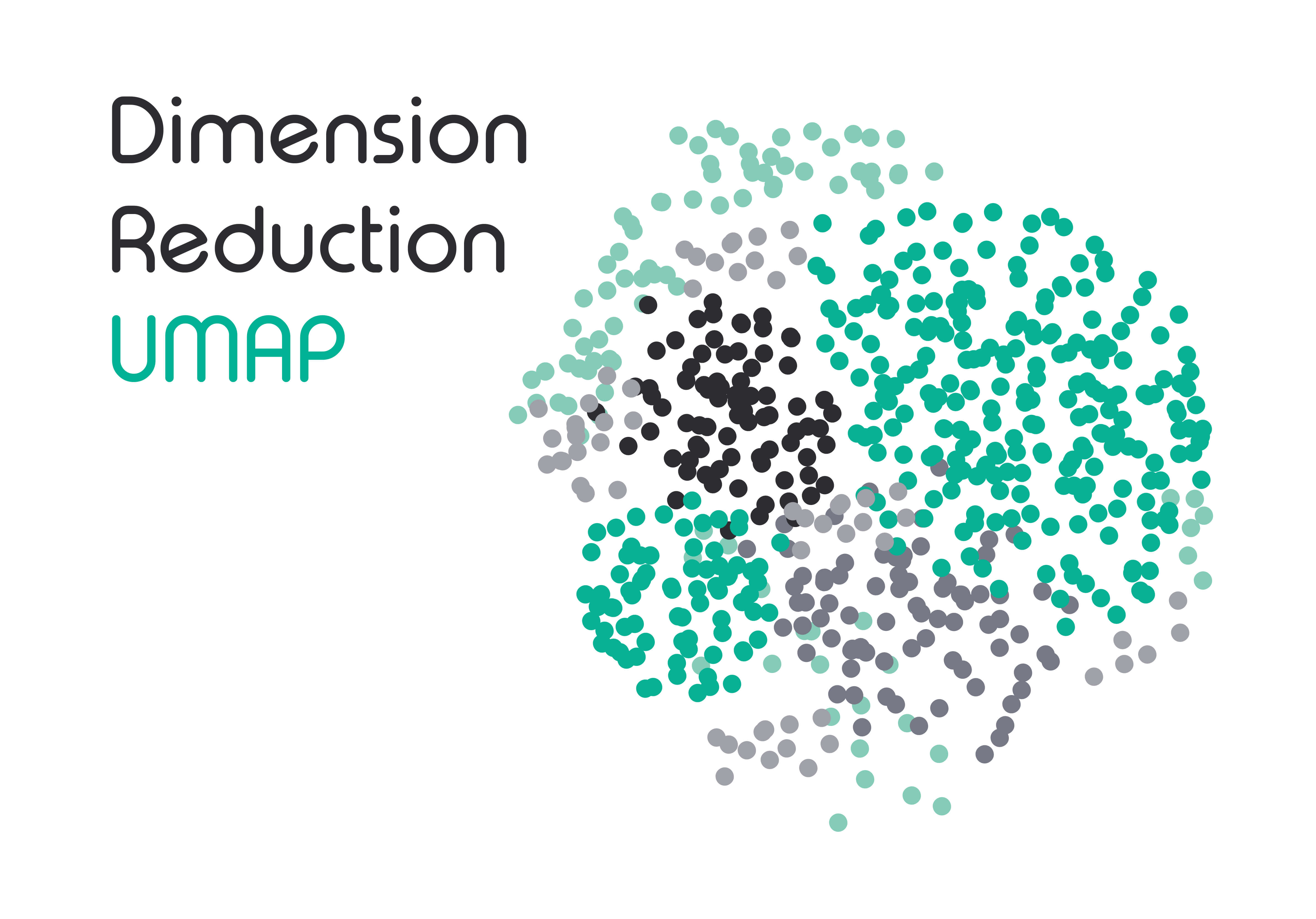
What is UMAP

Uniform Manifold Approximation and Projection (UMAP) was first described by McInnes et al. in 2018. At first glance, UMAP and t-SNE are highly similar to each other. UMAP can also be expressed in 4 equations, pretty much like those used in t-SNE to learn more read article 3 in this series. Both start with the construction of a high-dimensional representation of the data, then try to reconstruct a low-dimensional graphic that is as close to the first one as possible.

However, there are a few key differences:

• If t-SNE normalized data on both high- and low-dimensions, UMAP skips through these steps.
• Other mathematical changes (such as using k-nearest neighbor in lieu of perplexity equation, or Stochastic Gradient Descent in place of Gradient Descent) help UMAP reduce memory usage and shorten running time. The mathematical underpinning is interesting but is out of scope for this blog.
• The 4 main parameters that you should know about are: n_neighbors, min_dist, n_components, and metric. I will discuss the usage of each parameter in the next section.

UMAP pros

UMAP is a great nonlinear technique that tends to keep a more global structure of the dataset than t-SNE (but this is not without cons, see the following section). Furthermore, plots generated by UMAP are more continuous in nature compared to t-SNE helping it to display cell biological lineages better. Overall, data can be categorized as binary, categorical, and continuous whereby scRNA-Seq data tend to be continuous.

In t-SNE, one often tunes “perplexity”, a parameter that guesses the number of close neighbors each point has. In comparison, one tunes n_neighbours and min_dist in UMAP to balance local and global structures.

Unlike t-SNE which initializes randomly, UMAP does not, and thus running UMAP multiple times would generate the same results.
UMAP is rather light computationally. You can run UMAP on a strong laptop. For t-SNE, you likely need cluster computers.

UMAP cons

Interpretability of UMAP is lacking. The best method for interpretability is PCA. As its name alludes to, UMAP assumes a manifold data structure. To learn what a manifold is take a look at this article. UMAP then tends to find manifold structure within data noise. The larger the dataset, the less noise, hence UMAP is recommended for a big dataset but not small once.

Best practices for UMAP

When using UMAP, you should tune n_neighbors and min_dist to be suitable to your research question. I cannot comment precisely on how you should tune them, as this is a trial-and-error process that gets better with experience. The default values are 15 and 0.1 respectively.

In general, the rules are:

• n_neighbors values ranging from 2 (a very local view of the manifold) up to 200 (a quarter of the data). Tuning this parameter is a tradeoff between local versus global structure preservation.
• As min_dist is increased, the points are pushed apart into softer more general features, providing a better overarching view of the data at the loss of the more detailed topological structure. This also shows a tradeoff between local versus global structures.

You can also tune n_components in UMAP. It determines the number of dimensions in the lower-dimensional space. UMAP scales well in embedding dimension so n_components can be higher than 2 or 3 dimensions. This is an advantage of UMAP over t-SNE.

A detailed technical tutorial can be found on this website.

Conclusion

The three methods PCA, t-SNE, and UMAP all have their pros and cons. In general, for scRNA-Seq analysis, we would recommend the following:

• Perform quality control, feature selection and normalization on the count matrix. You can refer to this Seurat/R tutorial from Harvard University, here and here.
• Start your dimension reduction analysis with PCA. The default number of PCs is often between 30 and 50 but it’s best if you referred to the Scree plot to determine the exact plateau.
• If global structure preservation is your goal, use PCA only. It is excellent at reducing the dimensionality of your dataset.
• However, if interpretation and local structure are important, PCA will likely be problematic. You will then need to look at t-SNE or UMAP.
• Use PCA + t-SNE on a smaller dataset.
• Use PCA + UMAP on a bigger dataset.

The content of these blogs is meant to be introductory. If you need more resources, I suggest the following:

UMAP tutorial

HBC scRNA-Seq tutorial

Becht, E., McInnes, L., Healy, J. et al. Dimensionality reduction for visualizing single-cell data using UMAP. Nat Biotechnol 37, 38–44 (2019). 

McInnes, L., Healy, J., Melville, J. (2018) UMAP: Uniform Manifold Approximation and Projection for Dimension Reduction. ArXiv. 

If you need scRNA-seq-related help, Dolomite Bio offers end-to-end Single-Cell Consultancy Service that helps you through one or more steps of the workflow:

• Sample preparation
• Library preparation
• Sequencing
• Computational Analysis

Interested queries and/or suggestions for what we should write next in our blog series should be directed to: bioinformatics@dolomite-bio.com

Need help with your single cell data analysis? Check out Dolomite Bio’s new Bioinformatics Service