There is a wealth of analysis options for single cell data out there, which can be daunting for new users. We will discuss two popular pipelines that are tailored to biologists with some computational knowledge. This entails pre-processing through command line on computer terminals. The result can be a gene expression matrix (GEX) or Seurat object, which can be passed on to interactive post-processing software.
Based on popularity and credibility, the chosen pipelines are dropSeqPipe and kb-python, featuring two popular mappers (STAR and Kallisto) with comparison of ease-of-use, time, and memory consumption, as well as why and when to use them.
INDEX
- An introduction to single cell data
- Why dropSeqPipe and Kallisto- bustools?
- What are the differences in components of the two pipelines?
- What are the differences in time consumption and memory usage?
- Which pipeline is easier to use?
- What about the outputs?
- Which workflow should I use?
- Conclusion
- Further useful resources
An introduction to single cell data
Single cell RNA-Sequencing (scRNA-Seq), first published in 2009 (1), is an innovative technology in genomics, allowing for the measurement of transcript levels of single cells within a given sample.
Over the years, many methods for cell isolation have been developed and one of the most popular advancements were droplet-based scRNA-Seq technologies such as dropseq (2) or inDrop (3).
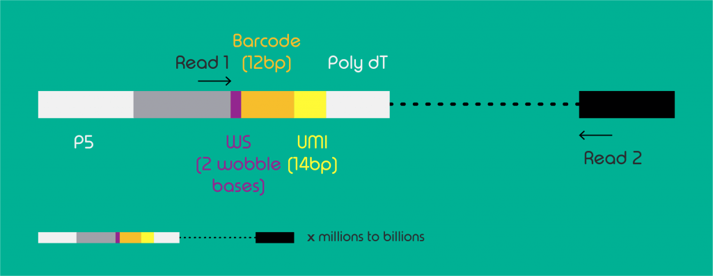
These methods can generate higher throughput compared to others, allowing for analysis of mRNA expression in thousands of individual cells at once. In this technology, 3’ sequencing is usually applied to cellular transcripts (4). Each transcript is uniquely tagged with an UMI (Unique Molecular Identifiers) and a barcode, thus differentiating transcripts of the same gene and those of different cells, respectively (5).

A single cell data set from droplet-based technologies will most commonly contain FASTQ files for 3 reads per gene. As depicted in figure 1, read 1 will contain information on the UMI and barcode sequencing, read 2 the transcript sequence and the third read the index.
The analysis of such data can roughly be divided into 3 phases, pre-alignment and alignment, which are part of the pre-processing workflows discussed here, and post-alignment steps dedicated to extracting meaningful information of your data.
Within pre-processing there are several important steps such as quality control of data, removal of adapters, barcode demultiplexing and deduplication (6,7).
Learn more about How to quality control your scRNA-seq data here.
The final pre-processing step is read alignment against a reference genome or transcriptome. Mapping of reads has a significant influence on the result of the data analysis and sequence mappers have been developed to a great extent. Pipelines discussed in the following chapters mostly differentiate in the mappers different functionalities.
Why dropSeqPipe and Kallisto-bustools?
The available tools can broadly be categorized into alignment-based and alignment-free, also known as pseudo-alignment-based tools. Alignment-based tools are traditional approaches that infer sequence origin at their matched loci in the reference genome. On the contrary, pseudo-alignment is a fairly new approach that infers sequence origin by most potential loci based on k-mers counting (8) and sophisticated algorithms (specifically hash function) aligning it to a reference transcriptome. To make pre-processing less arduous, many integrated workflows have been created.
In this blog, we will compare dropSeqPipe, a commonly practiced workflow using alignment-based mapping tool STAR, and Kallisto-bustools (kb-python), featuring Kallisto, a new computationally innovative method based on a pseudo-alignment mapping.
What are the differences in components of the two pipelines?
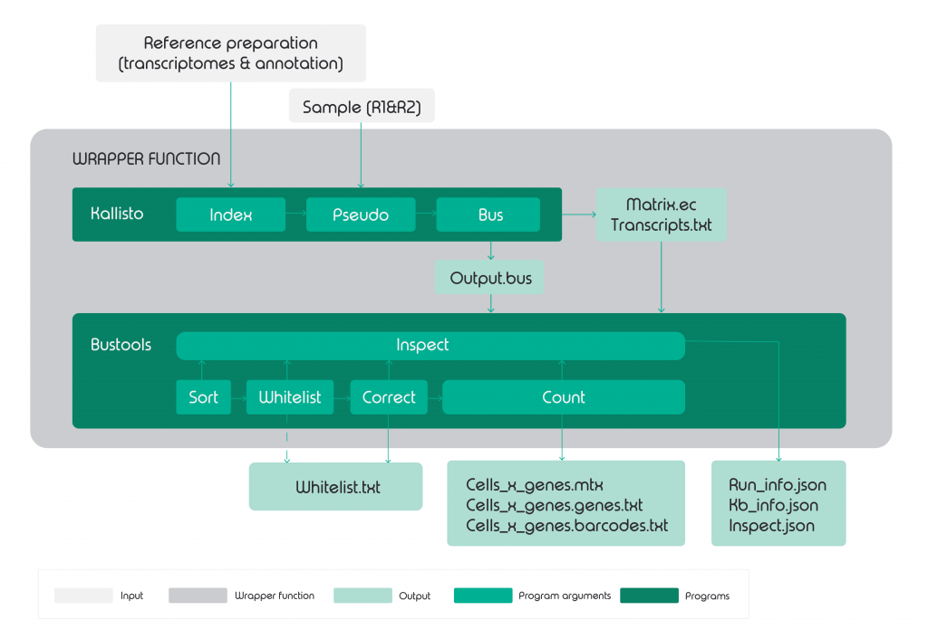
Kb-python is minimized to only core components – Kallisto (mapper) and BUStools. Designed for pseudoalignment, Melsted et al. (9) introduced a new mapping format called BUS (Barcode,UMI, Set) along with the bustools designed for BUS manipulation. The pipeline was constructed by wrapper functions wrapping Kallisto and bustools along with other supportive functions as displayed in figure 2.

On the other hand, given how widely dropSeqPipe featuring STAR as an alignment tool has been applied, it is fully equipped with additional programs for quality control. Starting from read quality control, cleaning input data for alignment, through to alignment and mapping and ending with matrices produced alongside log files to track each programs performance and reports.
To ensure all programs of the different platforms run harmoniously with controlled parameters and have robust performance over many tries, dropSeqPipe is built using a Workflow Management System (WMS) called snakemake. It is one of the most popular WMS in the bioinformatics community that is implemented in Python.
The advantage of using a workflow management system is that all program parameters are listed in a single file giving more clarity for all integrated programs. It also allows reproducible and scalable data analyses and can be seamlessly scaled to server, cluster, grid and cloud environments, without the need to modify the workflow definition.
In short, dropSeqPipe is structurally more complicated than kb-python but better equipped considering all aspects of pre-processing.

What are the differences in time consumption and memory usage?
Speed and memory-efficiency are undoubtedly the biggest and most significant advantages of kb-python. This is achieved through a simple pipeline build and the use of pseudoalignment. In a study by Du et al. (10), Kallisto has been shown to perform 4 times quicker with 7.7 times more efficiency in memory usage compared to STAR. Despite the tendency to miss more genes and lower correlations with the smRNA-FISH experiment for accuracy measure, Kallisto has been shown to be of high quality (11).
Which pipeline is easier to use?
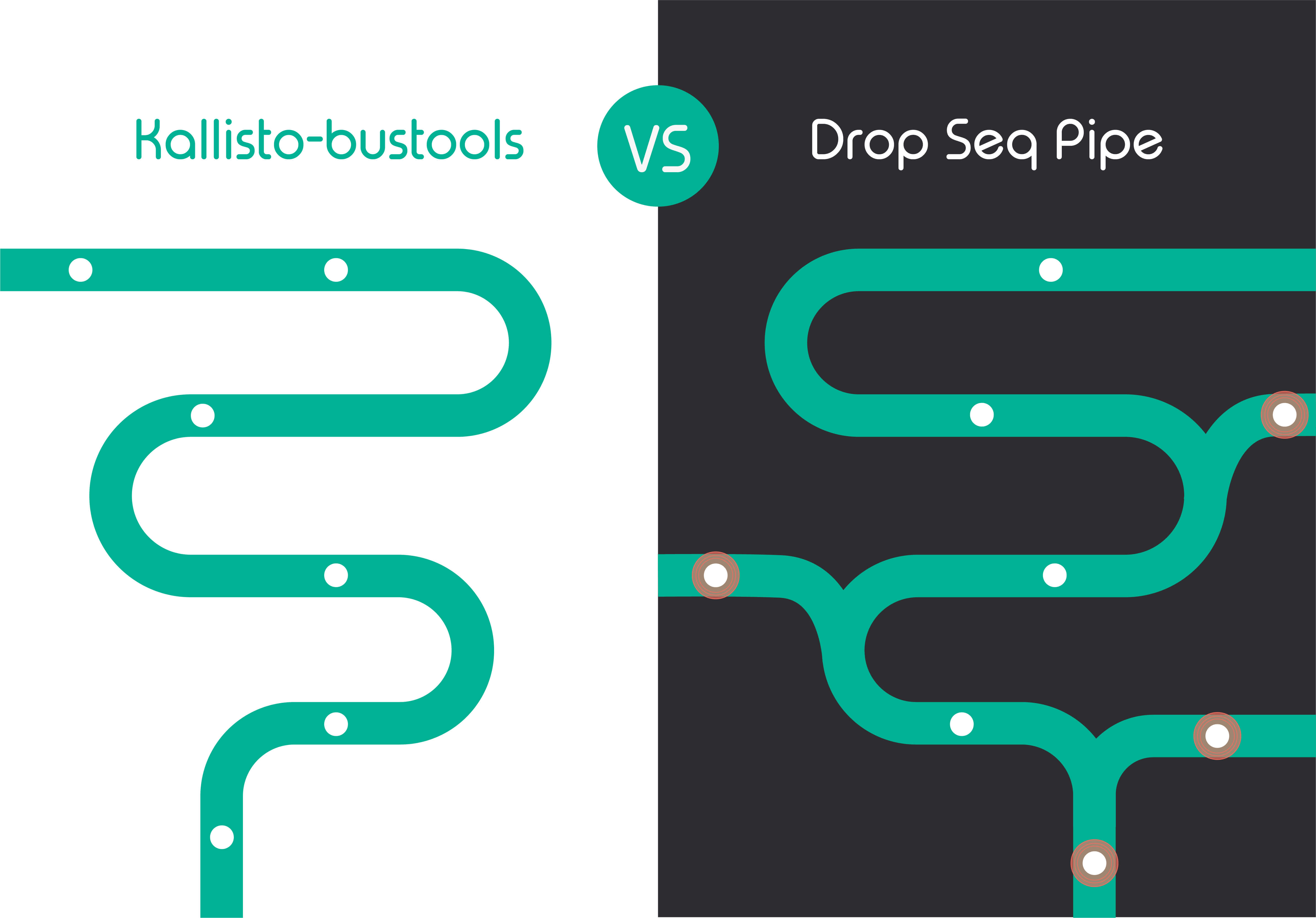
With a simple structure and only two commands to call throughout the whole pipeline, I personally think kb-python takes less time to get familiar with.
The first command prepares a pre-indexed transcriptome and a transcript-to-gene file, containing hashed kmers of the reference transcriptome and information on gene isoforms, respectively. This index only needs to be generated once. In a second step, Kallisto performs quantification by using your libraries (which consist of the FASTQ files as shown in Figure 1) by aligning it against the self-generated transcriptome.
The rest of the workflow is done with the second command, which involves barcode filtering, barcode collapsing, pseudo-alignment, and expression quantification. They are automatically run without much intervention.
DropSeqPipe can also run everything automatically and smoothly, given that you have prepared all as required.
Check out our blog on a quick guide to using dSP. Because dropSeqPipe packs many programs of many platforms into snakemake, everything needs to run by snakemake rules. Pay extra attention while preparing the following components (Table 1).
Table 1. Components of dropSeqPipe
| # | Component | Role | Source | Note |
| 1 | config.yaml
(Must be in working directory) |
Decide all the parameters for each program of dropSeqPipe | */dropSeqPipe/templates | Need modification |
| 2 | sample.csv | Identify all the samples | */dropSeqPipe/templates | Need modification |
| 3 | gtf_biotypes.yaml | Gene structures information (.gtf) | */dropSeqPipe/templates | Can be customised |
| 4 | adapterfile.fa | Adapters from sequencing platforms | */dropSeqPipe/templates | Can be customised |
| 5 | Input data
(a subdirectory) |
The FastQ files (sequences of transcripts) – core data of the whole pipeline | Put your raw data here. | Can be customised |
Put these 5 items into one directory that you define as working directory or carefully state their location in the config.yaml so that snakemake knows where to find them. To run the workflow, make sure you set up your working directory appropriately and check if it is in the dropSeqPipe folder that was cloned to your computer from github. This will ensure that your computer can find the program snakemake, Snakefile and all the rules used to build dropSeqPipe. This part does take some getting used to and isn’t intuitive at first. Once familiar with this folder it does help in understand the workflow and it is a very convenient system after all. Plus, the rules can be run separately which personally I think is a cool feature of snakemake.
What about the outputs?
Both pipelines produce the gene expression matrix (GEX) in the form of mtx (dropseqpipe) or mtx/h5ad/loom for kb-python. This is a central result that can be further processed by various other packages such as Seurat or Scanpy.
Results from kb-python are pretty straightforward. Aside from BUS files that come from pseudoalignment, matrices can be produced as normal gene count matrices in combination with a loom file, a h5ad, or as transcript-compatibility read count (TCC) (12,13). TCC is fairly new and is optimized for differential expression analysis – a valuable downstream analysis. Benchmarks against other methods show that they are reliable results (10,14–16).
In addition, statistics like total number of reads and barcodes from input files, number, and percentage of chosen barcodes in whitelists, means and medians of reads or UMIs per cell are calculated aiding the evaluation of the quality of the experiment. Post-processing the outputs from kb-python needs to be done manually, requiring skills in tools such as R (Seurat, SCE) or Python (Scanpy).
On the other hand, dropSeqPipe is pretty user interactive. It makes use of MultiQC – a program that integrates results of different samples into one to facilitate comparison of data quality between samples. Table 2 gives a comprehensive overview of all outputs generated by running dSP automatically.
Table 2. Summary of dSP outputs.
| Output | Content | Usage |
| logs | Log files for bbmap, cutadapt, dropseq_tools, fastqc | Input for visualisation and MultiQC. |
| reports | Multi-QC reports fastqc barcodes and reads data | Statistics of fastqc results from R1 and R2 files of all samples. |
| Multi-QC reports for barcodes and RNA filtering data | Statistics of cutadapt results (trimmed reads and adapter contents) from R1 and R2 files of all samples | |
| Multi-QC reports of STAR alignments | Statistics of STAR results (filtered, multi mapped, unmapped and uniquely mapped reads) of all samples | |
| Plots (visualization of log files) | Knee plots | Plot barcodes quality by number of reads (cumulative sum of reads in barcodes). |
| rna metrics plot | Plot barcodes quality by gene components (percentage of overlapping reads, intergenic reads, UTR reads, ribosomal reads, intronic reads and coding reads) | |
| violin plot (Figure 5) | Plot barcodes quality by their distribution in certain parameters. | |
| yield plot | Plot reads quality by number and percentage of filtered, multi mapped, unmapped and uniquely mapped reads | |
| adapter content plot | Plot adapter contents of samples | |
| Count vs UMI vs genes plots (Figure 4) | Correlation of count vs UMI troubleshoot technical amplification | |
| samples | Outputs of each samples | Extract trimmed R1 and R2 files, barcode list, BAM files, Splice Junction file, read and umi matrices of separated samples. |
| summary | Summary matrix and Seurat object. | Extract summarized matrices and Seurat object for post-processing. |


Which workflow should I use?
Depending on what you need from a bioinformatic pipeline either kb-python or dropSeqPipe will be the better choice.
If you are interested in isoforms of a transcript and are having data from single nuclei, either workflow will be able to analyze your data. Despite what you might expect kb-python is able to build reference transcriptomes that do contain intron information. In contrast, if your project requires detection of gene variants, SNPs or other methods that require inspection of base matches and mismatches to the genome, workflows that feature traditional alignment (such as dropSepPipe) are preferable.
Pseudo-alignment is optimized to solely answer the question of what was expressed. The answer lies in the most potential transcripts calculated. This lightweight algorithm is a perfect match for sole transcript quantification.
If you want to discover novel genes and transcripts or splice forms, STAR would be a better choice as the reads are aligned to genomes by algorithm optimized for keeping tracks of exons and introns by breaking reads into smaller pieces when unmappable (17). This means less dependence on the information of transcriptomes.
Results from Kallisto are stored in BUS files, which is a format that is specifically designed for pseudo-alignment and is limited to bustools. Meanwhile, DropSeqPipe results are stored in SAM/BAM files. which are extensive with the actual locations and mismatches of reads. They can be viewed in a genome browser and there are several independent tools to work with them.
Summary table
| dropSeqPipe | kb-python | |
| Mapping method | STAR: well-known, routinely used | Kallisto: new, innovative |
| Accuracy | ||
| Time and PC resources consumption |
X |
|
| Alignment references | Genomes | Transcriptome |
| scRNA-Seq data | ||
| sNuc–Seq data | ||
| Novel splice junction, gene, transcript or SNP detection |
X |
|
| Automation | Tools controlled through single Workflow Management Systems | Only two commands to call |
| Mapping output format | SAM/BAM files
– common format used by many programs – more informative => better for downstream analysis (splice junction, SNPs) |
BUS files
– new format, specifically for pseudoalignment |
| Matrix output | UMI and read count matrix in MTX format
Optional generation of Seurat or SingleCellExperiment objects |
UMI counts matrix in MTX format, TCC matrix with h5ad files or loom files for additional information (batch/samples/time) |
| Statistics and tables | ||
| Visualization of QC |
X |
Conclusion
In general, dropSeqPipe is a classic pipeline with many well-tested tools for scRNA-Seq data pre-processing. Despite the time-consuming performance, dropSeqPipe allows for visualization of many control metrics that are practical for users. Plus, it allows for more complex data analysis than just gene expression.
Meanwhile, kb-python is an innovative tool with several advancements in the computational methods used. The tool has been benchmarked against both traditional and current lightweight algorithms, which show favorable results with significant reduction in memory usage and time consumption (10,14–16). We would highly recommend it as a tool for single cell data analysis when all you are looking for is a fast gene expression analysis and are able to produce plots for quality control yourself.
If you are interested in reading more about pre-processing tools, here are some recommendations:
1. Tang F, Barbacioru C, Wang Y, Nordman E, Lee C, Xu N, et al. mRNA-Seq whole-transcriptome analysis of a single cell. Nat Methods. 2009 May;6(5):377–82.
2. Macosko EZ, Basu A, Satija R, Nemesh J, Shekhar K, Goldman M, et al. Highly Parallel Genome-wide Expression Profiling of Individual Cells Using Nanoliter Droplets. Cell. 2015 May 21;161(5):1202–14.
3. Klein AM, Mazutis L, Akartuna I, Tallapragada N, Veres A, Li V, et al. Droplet barcoding for single cell transcriptomics applied to embryonic stem cells. Cell. 2015 May 21;161(5):1187–201.
4. Ma F, Fuqua BK, Hasin Y, Yukhtman C, Vulpe CD, Lusis AJ, et al. A comparison between whole transcript and 3’ RNA sequencing methods using Kapa and Lexogen library preparation methods. BMC Genomics. 2019 Jan 7;20(1):9.
5. Chen G, Ning B, Shi T. Single-Cell RNA-Seq Technologies and Related Computational Data Analysis. Front Genet. 2019;10:317.
6. He B, Zhu R, Yang H, Lu Q, Wang W, Song L, et al. Assessing the Impact of Data Preprocessing on Analyzing Next Generation Sequencing Data. Front Bioeng Biotechnol. 2020;8:817.
7. Martin M. Cutadapt removes adapter sequences from high-throughput sequencing reads. EMBnet.journal. 2011 May 2;17(1):10.
8. Manekar SC, Sathe SR. A benchmark study of k-mer counting methods for high-throughput sequencing. GigaScience. 2018 Dec 1;7(12):giy125.
9. Melsted P, Ntranos V, Pachter L. The barcode, UMI, set format and BUStools. Bioinformatics. 2019 Nov 1;35(21):4472–3.
10. Du Y, Huang Q, Arisdakessian C, Garmire LX. Evaluation of STAR and Kallisto on Single Cell RNA-Seq Data Alignment. G3 Bethesda Md. 2020 May 4;10(5):1775–83.
11. Sahraeian SME, Mohiyuddin M, Sebra R, Tilgner H, Afshar PT, Au KF, et al. Gaining comprehensive biological insight into the transcriptome by performing a broad-spectrum RNA-seq analysis. Nat Commun. 2017 Jul 5;8(1):59.
12. Ntranos V, Kamath GM, Zhang JM, Pachter L, Tse DN. Fast and accurate single-cell RNA-seq analysis by clustering of transcript-compatibility counts. Genome Biol. 2016 May 26;17(1):112.
13. Tang M, Sun J, Shimizu K, Kadota K. Evaluation of methods for differential expression analysis on multi-group RNA-seq count data. BMC Bioinformatics. 2015 Nov 4;16(1):360.
14. Srivastava A, Malik L, Sarkar H, Zakeri M, Almodaresi F, Soneson C, et al. Alignment and mapping methodology influence transcript abundance estimation. Genome Biol. 2020 Sep 7;21(1):239.
15. Zheng H, Brennan K, Hernaez M, Gevaert O. Benchmark of long non-coding RNA quantification for RNA sequencing of cancer samples. GigaScience. 2019 Dec 1;8(12):giz145.
16. Everaert C, Luypaert M, Maag JLV, Cheng QX, Dinger ME, Hellemans J, et al. Benchmarking of RNA-sequencing analysis workflows using whole-transcriptome RT-qPCR expression data. Sci Rep. 2017 May 8;7(1):1559.
17. Dobin A, Davis CA, Schlesinger F, Drenkow J, Zaleski C, Jha S, et al. STAR: ultrafast universal RNA-seq aligner. Bioinformatics. 2013 Jan;29(1):15–21.

