A guide to quality controlling your scRNA-Seq data

How to quality control your single cell RNA-seq data

Why data quality control is important

Low-quality libraries in single cell RNA-seq (scRNA-seq) data can originate from a variety of experimental factors, such as damaged or stressed cells, or failures in library preparation. The consequences are, typically, cells with low read counts, with few detected genes and high levels of mitochondrial RNA. These low-quality cells can bias the overall analysis for a given dataset and generate misleading results.

Data quality is paramount when it comes to the analysis and interpretation of single cell data. It is therefore of utmost importance to take a few steps to check data quality before proceeding with in-depth analysis.

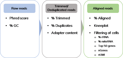
In this blog post, I will summarize some of the quality control measures that can be used and the methods that can be employed, to remove low quality cells from datasets (Figure 1).

Index:  

Step 1: Assessing the read quality of your sequencing data 
Step 2: Adapter trimming and de-duplication of reads -keeping what you need
Step 3: Quality read out after alignment
Step 4- Useful features to weed out the unwanted cells. 

Step 1: assessing the read quality of your sequencing data

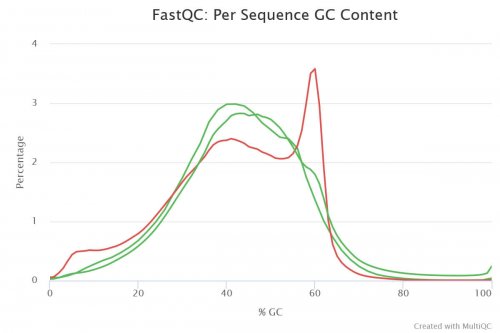
Once you have obtained your sequencing data, the first thing you want to do is to check read quality. A very commonly used quality control tool is FastQC. It returns quality metrics from sequencing data for both single-cell and bulk RNA-seq data (1). With a tool called MultiQC, those results can be nicely visualized and compared between samples (2). A variety of different quality control metrics are displayed, two of which are the GC content and the Phred score.

The GC content is distinct for each species and can be an indicator of sample contamination. Human genomes, for example, have a mean GC content of about 41%. If your detected value is notably different from what you would expect, the sample might have been contaminated (3). In a standard library, you would expect to see a normal distribution of GC content where the curve peaks at a value corresponding to the overall GC content of the underlying genome (green lines, Figure 2). An unusually shaped distribution or a secondary peak would indicate a contamination. Depending on the shape of the secondary peak it might either be a contamination with a different species (broader peak) or adapter dimers (sharper peak as shown with the red curve in Figure 2) (4).

The sequence quality score, also called a Phred score, is an indication of the average quality of the sequencing reads (5). In general, low quality scores are pretty rare and scores above 28 are the norm. However, if the run quality overall is quite low (below 20) it could indicate a systematic problem during sequencing, such as poor imaging of DNA clusters or a problem with a flow cell.

Step 2: Adapter trimming and de-duplication of reads – keeping what you need

Once you have checked that the quality of your library is adequate, there is one more thing to do before aligning your reads to the reference genome. This step involves the trimming of any unwanted sequences and de-duplication of reads.

Trimming is done to remove, for instance, adapters or low-quality sequences from the end of reads. In dropSeqPipe (dSP, see our blog post “Keep calm and dropSeqPipe” for more information), adapters and their sequences are predefined in a file called ‘adapters.fa’. Trimmable sequences include Illumina-specific adapters and transcripts or Drop-seq specific adapters. During scRNA-Seq, ligation of adapters prior to sequencing is necessary for library amplification, immobilization on the flow cell and sequencing.

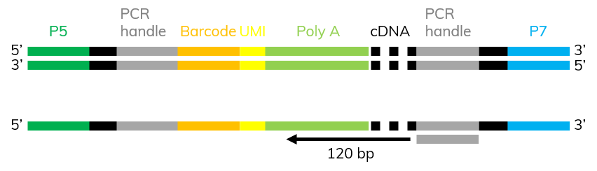
If adapters are sequenced during NGS, reads have extended over the actually transcript into the adapters and polyA tail at the 3’prime end (Figure 3). This is fairly common in scRNA-seq, as cDNA fragments are most commonly short. Adapter contamination leads to alignment errors as they are artificial sequences that are not present in the reference genome. This makes adapter trimming necessary to avoid a high percentage of unaligned reads in your dataset.

PCR duplicates are a major challenge in any method that involves sequencing, as much sequencing power can end up being wasted on identical copies of the same transcript. This is especially true for scRNA-seq as this method necessarily begins with very low quantities of mRNA that might lead to over amplification of the cDNA during PCR. Luckily, most single-cell applications utilize a short sequence in their oligo capture probe, called a unique molecular identifier (UMI), that allows for detection of PCR duplicates. UMIs are used to tag each individual transcript from the moment they are captured to help identify unique reads later in the analysis process. During data analysis, tools like SAMTools or Picard detect identical reads that are associated with the same UMI and barcode, and discard all but one copy (6).

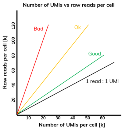
The dSP workflow (see our blog post “Keep calm and dropSeqPipe” for more information) generates a graph that plots the number of UMIs per cell against the number of reads per cell (Figure 4). The black line in this graph represents the ideal ratio of UMIs to reads (1:1), representing no PCR duplication. The closer your samples align to this line, the less duplication occurred as part of your chosen process. Duplication mostly happens during the scRNA-Seq protocol’s PCR steps, including cDNA amplification and amplification during Nextera library preparation. Some degree of duplication is inevitable during those steps, but it should be kept to a minimum to avoid unnecessary read loss. Typically, if you have more then 30 – 40% of duplicates it is worthwhile investigating whether your workflow could potentially be optimized.

So, what are the reasons for overamplification? The most obvious one is working with too low concentrations of starting material. This can happen if your chosen cell type has very low transcription levels or if you have not amplified your cDNA enough prior to library preparation. Both cases lead to library overamplification and thereby generation of duplicates. Problems also arise when fragment sizes within your library are too variable. Smaller fragments will be overrepresented as they are easier to amplify. To increase the amount of starting material, you might want to increase lysis time or change the lysis buffer composition to improve both cell lysis and mRNA capture.

If a low quantity of starting material is inherent to your sample type, such as in nuclei, changing the droplet size might be the way to go. In DroNc-seq (or sNuc-seq) reducing the droplet size results in higher concentration of mRNA and thereby increased captured of transcripts (7). As biologists, we don’t always get to choose the samples and cell types we use. An inherently transcriptionally-inactive cell type may require us to increase the number of PCR cycles to amplify enough material for a meaningful library.

Step 3: Quality read out after alignment

Following trimming and quality control of reads, these need to be mapped to the reference genome using tools like STAR. This step is called alignment and is required to identify genes that in the case of scRNA-Seq are differentially expressed between samples. Expression levels and differentially-expressed genes can then be used to identify low-quality barcodes (cells) and remove them from the subsequent data analysis.

Doublet rate and hidden multiples

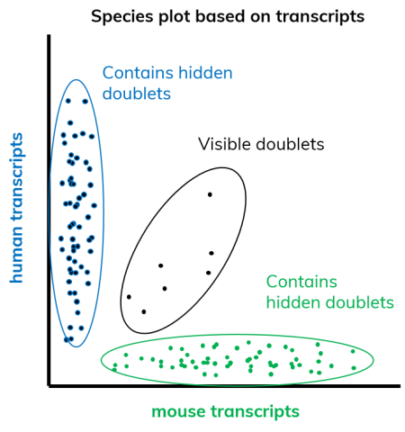
There are many indicators of a good quality dataset and many parameters to look out for, one of which is the doublet rate. The doublet rate refers to the frequency at which multiple cells are encapsulated alongside a bead. The doublet rate can be determined using a mixed-species experiment. In such an experiment, human and mouse cells are dropletized at a 1:1 ratio and the number of transcripts, or genes, detected for each species for every given barcode (i.e. cell) are plotted in what is called a Barnyard plot (Figure 5). In the dSP workflow (see our blog post “Keep calm and dropSeqPipe” for more information) multiplets are defined by their ratio of mouse to human transcripts. If the mixing of one species with another exceeds 20% the cell is typically classified as a multiplet.

When calculating the doublet rate, the number of multiples is divided by the total cell count. The resulting number accounts for the “visible” doublet rate (mixed species doublets) only. In order to adjust for doublets of the same species, this number needs to be doubled (Figure 5). Whilst mouse-mouse and human-human doublet are functionally invisible in this assay, their rate of occurrence is predictably the same as that of the visible mouse-human and human-mouse multiplets.

Doublet rates in microfluidic systems are, among other aspects, mainly influenced by the number of cells encapsulated per sample. Therefore, if you happen to hear about doublet rates that sound too good to be true, check first how much cells are actually being encapsulated. Frequently in literature, doublet rates can be artificially lowered by simply loading a decreased concentration of starting cells. Typically, if running standard cell lines at a dilution of one cell per twenty droplets, you can expect doublet rates between 4 and 7%.

Step 4: Useful features to weed out the unwanted cells.

Determining the number of detected cells

A unique aspect of scRNA-seq in droplets, as on the Nadia Instrument, is that we do not know whether a particular barcode corresponds to a cell-containing or an “empty” droplet. Therefore, we need to differentiate cells from empty droplets based on the number of reads detected. This, however, is difficult as empty droplets can contain ambient (i.e., resulting from early cell lysis) RNA that can be captured and sequenced, resulting in low-level read counts for barcodes that have not actually captured a single cell transcriptome.

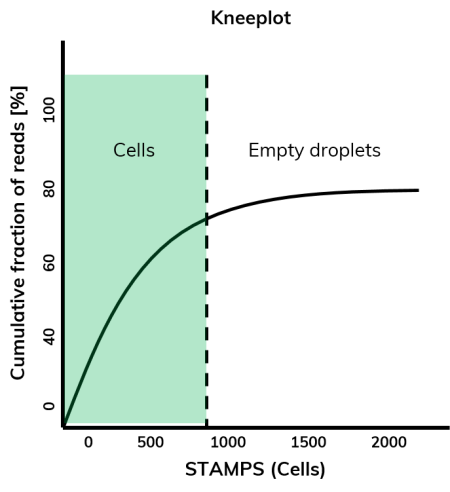
Fortunately, there are two plots that make it easier to estimate the real number of cells: the cumulative distribution plot and the barcode rank plot (8). The cumulative distribution plot, also called kneeplot, plots the cumulative fraction of reads against cell barcodes in descending order (Figure 6), exhibiting a sharp (most of the time, anyway!) transition between barcodes with large and small total counts, called the knee or inflection point. Any barcode left of the inflection point is regarded as a cell-associated barcode and any barcode on the right is associated with an empty droplet.

This plot is automatically generated by the dSP workflow. The barcode rank plot arranges cell barcodes by descending read count and plots them against the number of reads using a log scale on both axes. The resulting plot shows an inverse S-curve, where the drop indicates the separation between cells captured by a bead and empty beads (8).

However, this can lead to the exclusion of cells that have very low RNA content or include well-sequenced empty droplets. To distinguish these instances, you can test whether the expression profile of a cell barcode is significantly different from the ambient mRNA pool. A tool called ‘emptyDrops’ uses exactly this method to determine whether a barcode corresponds to a cell-containing droplet or not (9).

Most often, background mRNA contamination can be minimized experimentally by ensuring high levels of viability in your initial single cell isolate.

Amount of rRNA and mitoRNA as indicator of overall cell health

Looking at the percentage of mitochondrial and ribosomal RNA is another great way of filtering out unwanted cells. The threshold in terms of number of reads attributed to these parameters varies depending on cell type and health state. High mitochondrial transcript levels can be an indicator of cellular stress, which alters the transcriptome significantly towards the expression of stress related genes and thereby biases the final clustering results. It is therefore recommended to exclude cells with high mitochondrial RNA levels from the analysis.

Numbers, however, should be taken with a pinch of salt as they depend upon cell types, similarly to expression levels. Cell types like cardiomyocytes or hepatocytes have very high levels of mitochondrial RNA due to their high metabolic activity (10). As a comparison, in a healthy heart muscle cell you would expect about 30% mitochondrial RNA. The same number for a lymphocyte, however, would indicate high levels of cell stress (10).

Top 50 genes and nUMI/ nGene

In addition to the QCs described above, dSP also produces a plot that shows the percentage of reads that belong to the 50 most expressed genes. This feature is valuable to detect genes that are overabundant and therefore might drive most of the variation in a given dataset. In a typical scRNA-seq on Nadia experiment, we find the majority of samples to have values from 5 to 20%.

Similarly, a quite commonly used method of filtering cells is to look at the number of transcripts (UMIs) or genes detected per cell. Typically, a researcher will define a threshold above or below which cells with either very high or very low transcription values will be discarded. Removing those cells from further analysis is beneficial as very high UMI numbers could indicate a doublet, and very low numbers usually result from poor mRNA capture (10).

Summary

Data and cell quality are key to unbiased data analysis. There are a number of QC steps involving raw NGS data as well as subsequent data processing that will result in reliable data quality (Figure 1). Pre-processing QC includes parameters such as the Phred score and the GC content. After trimming and de-duplication, reads can be aligned to the reference genome and linked to their respective barcode. Once the number of detected cells has been determined and one is happy with the pre-processing QC, filtering of cells can take place. Cell filtering is the last, but one of the more important, steps to remove low-quality transcriptomes that could potentially bias the overall data analysis and generate misleading results.

Literature

1. Wingett SW, Andrews S. FastQ Screen: A tool for multi-genome mapping and quality control. F1000Research. 2018;7:1338.
2. Ewels P, Magnusson M, Lundin S, Käller M. MultiQC: summarize analysis results for multiple tools and samples in a single report. Bioinformatics. 2016 Oct 1;32(19):3047–8.
3. Lander ES, Linton LM, Birren B, Nusbaum C, Zody MC, Baldwin J, et al. Initial sequencing and analysis of the human genome. Nature. 2001 Feb 15;409(6822):860–921.
4. Per Sequence GC Content [Internet]. [cited 2019 Nov 25]. Available from: https://www.bioinformatics.babraham.ac.uk/projects/fastqc/Help/3%20Analysis%20Modules/5%20Per%20Sequence%20GC%20Content.html
5. Ewing B, Hillier L, Wendl MC, Green P. Base-Calling of Automated Sequencer Traces UsingPhred. I. Accuracy Assessment. Genome Res. 1998 Jan 3;8(3):175–85.
6. Ebbert MTW, Wadsworth ME, Staley LA, Hoyt KL, Pickett B, Miller J, et al. Evaluating the necessity of PCR duplicate removal from next-generation sequencing data and a comparison of approaches. BMC Bioinformatics [Internet]. 2016 Jul 25 [cited 2019 Nov 18];17(Suppl 7). Available from: https://www.ncbi.nlm.nih.gov/pmc/articles/PMC4965708/
7. Habib N, Avraham-Davidi I, Basu A, Burks T, Shekhar K, Hofree M, et al. Massively parallel single-nucleus RNA-seq with DroNc-seq. Nat Methods. 2017 Oct;14(10):955–8.
8. Rich-Griffin C, Stechemesser A, Finch J, Lucas E, Ott S, Schäfer P. Single-Cell Transcriptomics: A High-Resolution Avenue for Plant Functional Genomics. Trends Plant Sci [Internet]. 2019 Nov 25 [cited 2019 Dec 11]; Available from: http://www.sciencedirect.com/science/article/pii/S1360138519302729
9. Lun ATL, Riesenfeld S, Andrews T, Dao TP, Gomes T, Marioni JC, et al. EmptyDrops: distinguishing cells from empty droplets in droplet-based single-cell RNA sequencing data. Genome Biol. 2019 Mar 22;20(1):63.
10. AlJanahi AA, Danielsen M, Dunbar CE. An Introduction to the Analysis of Single-Cell RNA-Sequencing Data. Mol Ther – Methods Clin Dev. 2018 Sep 21;10:189–96.