Visualizing single cell data using Seurat – a beginner’s guide
In the single cell field, large amounts of data are produced but bioinformaticians are scarce. Therefore, it is an important (and much sought-after) skill for biologists who are able take data into their own hands.
Luckily, there have been a range of tools developed that allow even data analysis noobs to get to grips with their single cell data. For a lot of us the obvious (and easiest) answer will be to use some form of guide user interface (GUI), such as those provided by companies like Partek (watch this webinar to learn more) that enables us to go from raw data all the way to visualization.
Although convenient, options offered for customization of analysis tools and plot appearance in GUI are somewhat limited. Combining dropSeqPipe (dSP) for pre-processing with Seurat for post-processing offers full control over data analysis and visualization.
The dSP pipeline with all its tools is designed to provide a reproducible, almost automatic, workflow that goes from raw reads (FASQ files) to basic data visualization. This is the point at which a specific experimental design requires manual intervention, for instance, when generating graphs. This is usually the exciting bit and it cannot be automated as requirements are often specific to a researcher’s needs.
dSP produces output that is tailored for a quasi-standard data visualization software in the single-cell world called Seurat and Scater. Seurat and Scater are package that can be used with the programming language R (learn some basic R here) enabling QC, analysis, and exploration of single-cell RNA-seq data. To help you get started with your very own dive into single cell and single nuclei RNA-Seq data analysis we compiled a tutorial on post-processing of data with R using Seurat tools from the famous Satija lab.
Index:
1. The tools you need to follow the tutorial
2. An Introduction to R studio and its features
3. Step 1: Downloading R and R studio
4. Step 2: Defining the working directory
5. Step 3: Extracting the meta data from the Seurat object
6. Step 4: Data QC
7. Step 5 – Normalizing the data
7. Step 6: Visualization of marker gene expression
8. Step 7: Dimension reduction plots
What tools will you need?
- An installed R and R studio package
- A Seurat object from one of your scRNA-Seq or sNuc-Seq projects.
- A computer…but that probably goes without saying
Don’t have any of this? (Well hopefully you’ll have the computer…we can’t help very much with that) but otherwise don’t you worry, you can find a detailed step by step introduction below on how to install R and R studio and we have placed a Seurat object here ready for you to download and play with.
Ticking all the boxes? Great! You can go straight to Step 1: Downloading R and R studio.
Disclaimer: This is for absolute beginners, if you are comfortable working with R and Seurat objects, I would suggest going to the Satija lab webpage straight away.
An Introduction to R studio and its features
If you have never used R, have a quick read of this introduction which familiarizes you with the most basic features of the program. There is plethora of analysis types that can be done with R and it is a very good skill to have! Intrigued? To learn more about R read this in depth guide to R by Nathaniel D. Phillips.
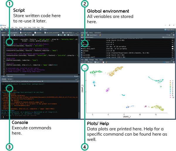
1. Script
Of course, you could write all your code in the console, however. none of that would be saved. Best practice is to save it in a script that will allow you to access it again once a new data set comes your way. Generally speaking, an R script is just a bunch of R code in a single file.
Writing a new script
To start writing a new R script in RStudio, click File – New File – R Script.
Execution of commands
If you would like to execute one of the commands in the script, just highlight the command and press Ctrl + Enter. You will see it appearing in the Console window.
Comments
Anything starting with a # is a comment, meaning that even if executed in the command line it won’t be read by R. It is simply helpful for the user to explain the purpose of the command that is written below.
2. Global environment
This is where R stores all the objects and variables created during a session. In the same location you can also find “History”, which lists all the commands executed during a session.
3. Console
This is the window in which you can type R commands, execute them and view the results (except plots). You can find some information on how to make your work with R more productive here.
4. Plots/ Help
This is the window in which R will print the plots generated and open the help tab if in the console ?function is executed.
Step 1: Downloading R and R studio
Start with installing R and R-Studio on your computer. Downloads for Windows and macOS can be found in the links below, install both files and run R studio. R will provide you with the necessary software to write and execute R commands, R studio is helpful as it provides a nice graphical interface for the daily use of R.
R download
Windows https://cran.r-project.org/bin/windows/base/
macOS https://cran.r-project.org/bin/macosx/
R Studio download
https://www.rstudio.com/products/rstudio/download/#download
Downloading a Seurat object
You can find a Seurat object here, which is some mouse lung scRNA-Seq from Nadia data for you to play with.
Installing relevant packages
When you first open R Studio it will pretty much be a blank page. Below are some packages that you will need to install to be able to use the code presented in this tutorial. This only needs to be done once after R is installed.
Note!: All code must be entered in the window labelled Console. Copy past the code at the > prompt and press enter, this will start the installation of the packages below. You will know that the script is completed if R displays a fresh > prompt in the console.
install.packages('BiocManager')
BiocManager::install('multtest')
install.packages('Seurat')
install.packages('dplyr')
Note: After installing BiocManager::install('multtest') R will ask to Update all/some/none? [a/s/n]: enter n to not update other packages.
Step 2: Defining the working directory
In order for R to find your Seurat object you will need to tell the program where it is saved, this location is called your working directory. This step will show you how to set this directory.
# Note you can copy the path from windows however you will have to change all \ to /
setwd("insert path")
Loading the relevant libraries
This step will install required packages and load relevant libraries for data analysis and visualization.
Note!: Libraries need to be loaded every time R is started
library(Seurat)
library(ggplot2)
library(dplyr)
library (patchwork)
Loading the Seurat object into R global environment
Its good practice to save every data set that is uploaded into R under a specific name (variable) in the global environment in R. This will allow you to transform or visualize that data simply by calling its variable. This is also true for the Seurat object when it is first loaded into R.
Note!: The Seurat object file must be saved in the working directory defined above, or else R won’t be able to find it.
#This loads the Seurat object into R and saves it in a variable called ‘seuratobj’ in the global environment
seuratobj <- readRDS("R_Seurat_objects_umap.rds")
Step 3: Extracting the meta data from the Seurat object
A Seurat object contains a lot of information including the count data and experimental meta data. The count data is saved as a so-called matrix within the seurat object, whereas, the meta data is saved as a data frame (something like a table). Meta data stores values such as numbers of genes and UMIs and cluster numbers for each cell (barcode). Just like with the Seurat object itself we can extract and save this data frame under a variable in the global environment.
#Saves the data frame meta data in a variable called ‘meta.data’ in the global environment
meta.data <- seuratobj@meta.data
Data frames are standard data types in R and there is a lot we can do with it. To learn more on what to do with data frames, have look here
#This will show you the first 7 lines of your data frame
head(meta.data)
orig.ident nCount_RNA nFeature_RNA           cellNames  samples    barcode expected_cells read_length
CT2_S249_AAAACTCACC   CT2_S249        784          628 CT2_S249_AAAACTCACC CT2_S249 AAAACTCACC            600         150
CT2_S249_AAAAGGTGTG   CT2_S249       1747         1114 CT2_S249_AAAAGGTGTG CT2_S249 AAAAGGTGTG            600         150
CT2_S249_AAAATCAATC   CT2_S249       3906         2134 CT2_S249_AAAATCAATC CT2_S249 AAAATCAATC            600         150
CT2_S249_AAAATTCTTA   CT2_S249       3344         1799 CT2_S249_AAAATTCTTA CT2_S249 AAAATTCTTA            600         150
CT2_S249_AAACAAAGGC   CT2_S249       5323         2732 CT2_S249_AAACAAAGGC CT2_S249 AAACAAAGGC            600         150
CT2_S249_AAACGACCGA   CT2_S249        906          658 CT2_S249_AAACGACCGA CT2_S249 AAACGACCGA            600         150
batch nCounts  pct.sribo  pct.lribo   pct.Ribo    pct.mito     top50 umi.per.gene RNA_snn_res.0.8
CT2_S249_AAAACTCACC   CT2   24665 0.02933673 0.01658163 0.04591837 0.005102041 0.1964286     1.248408               9
CT2_S249_AAAAGGTGTG   CT2   85066 0.05266171 0.04121351 0.09387521 0.024613623 0.2329708     1.568223               5
CT2_S249_AAAATCAATC   CT2  208598 0.03763441 0.04121864 0.07885305 0.012032770 0.1738351     1.830366               5
CT2_S249_AAAATTCTTA   CT2  187974 0.02601675 0.03887560 0.06489234 0.018540670 0.2221890     1.858810               5
CT2_S249_AAACAAAGGC   CT2  132907 0.02423445 0.02141649 0.04565095 0.009956791 0.1666354     1.948389               9
CT2_S249_AAACGACCGA   CT2   61304 0.02759382 0.04856512 0.07615894 0.014348786 0.2240618     1.376900               3
seurat_clusters
CT2_S249_AAAACTCACC               9
CT2_S249_AAAAGGTGTG               5
CT2_S249_AAAATCAATC               5
CT2_S249_AAAATTCTTA               5
CT2_S249_AAACAAAGGC               9
CT2_S249_AAACGACCGA               3
It is usually a good idea to play around and inspect the data, you can for example try str(meta.data) or View(meta.data). The example below allows you to check which samples are stored in the Seurat object.
# Show samples stored in the data frame
# orig.ident contains sample names
unique(meta.data$orig.ident)
[1] CT2_S249
Levels: CT2_S249
Step 4: Data QC
Before starting to dive deeper into your data its beneficial to take some time for selection and filtration of cells based on some QC metrics. This can be easily done with Seurat looking at common QC metrics such as:
- The number of unique genes/ UMIs detected in each cell.
- The percentage mitochondrial/ ribosomal reads per cell
Read more to this topic here under “Standard pre-processing workflow”.
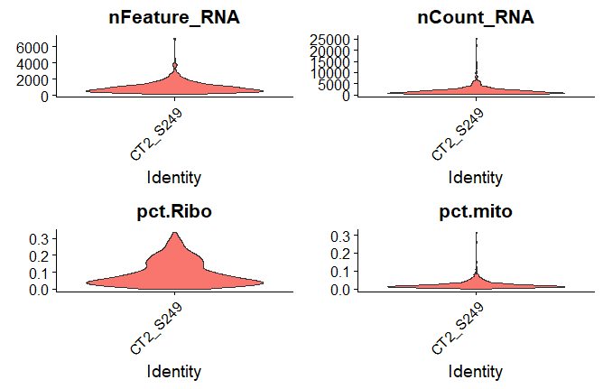
Violin plots
#Creates a violin plot for the number of UMIs ('nFeature_RNA'), the number of genes ('nCount_RNA'), % ribosomal RNA (‘pct.Ribo’) and % mitochondrial RNA (’pct.mito’) for each sample
VlnPlot(object = seuratobj, features = c('nFeature_RNA','nCount_RNA','pct.Ribo','pct.mito'), group.by = 'orig.ident',pt.size = 0,ncol=2)
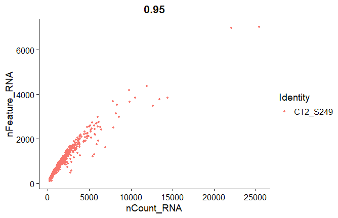
Scatter plots
# FeatureScatter can be used to visualize feature-feature relationships such as number of genes ("nFeature_RNA") vs number of UMIs ("nCount_RNA")
FeatureScatter(seuratobj, feature1 = "nCount_RNA", feature2 = "nFeature_RNA",group.by = 'orig.ident')
Step 5 – Normalizing the data
#LogNormalize (default) normalizes measurements for each cell by the total expression, multiplies by a scale factor of 10,000 by default
seuratobj <- NormalizeData(seuratobj, normalization.method = “LogNormalize”,scale.factor = 10000)```
Step 6 – Visualization of marker gene expression
Finding marker genes
# Finds all markers of cluster 1
cluster1.markers <- FindMarkers(seuratobj, ident.1 = 1, min.pct = 0.25)
|++++++++++++++++++++++++++++++++++++++++++++++++++| 100% elapsed=07s
# Shows top 5 markers genes of cluster 1
head(cluster1.markers, n = 5)
              p_val  avg_logFC pct.1 pct.2   p_val_adj
Cntn1  1.918870e-07  2.3485859   0.3 0.026 0.004927659
Sftpa1 2.927622e-04  1.7821664   0.5 0.141 1.000000000
Tmsb10 3.797597e-04 -2.9132579   0.0 0.637 1.000000000
B2m    3.827411e-04 -0.9140352   0.1 0.831 1.000000000
Tpm3   5.451834e-04 -2.3310006   0.0 0.617 1.000000000
Define set of marker genes
In order to create dot plots, heat maps or feature plots a list of genes of interests (features) need to be defined.
features <- c("Scgb1a1","Cd79b","Mzb1","Plac8","Trbc2","Cd8b1","Cd4","Cd3e","Cd3d","Tmem100","Vwf","Ednrb","Pecam1","Col1a2","Inmt","Dcn","Itgam","Itgax","C1qb","Sftpd","Sftpb","Sftpc","Foxj1","Scgb3a2","Ear2","Ager","Hopx","Pdpn","Rtkn2","Igfbp2")
Scaling data
Scaling, or linear transformation, is a standard pre-processing step prior to dimension reduction techniques.
all.genes <- rownames(seuratobj)
seuratobj <- ScaleData(seuratobj, features = all.genes)
Note: Scaling also helps make sure that highly-expressed genes don’t dominate the heat map.
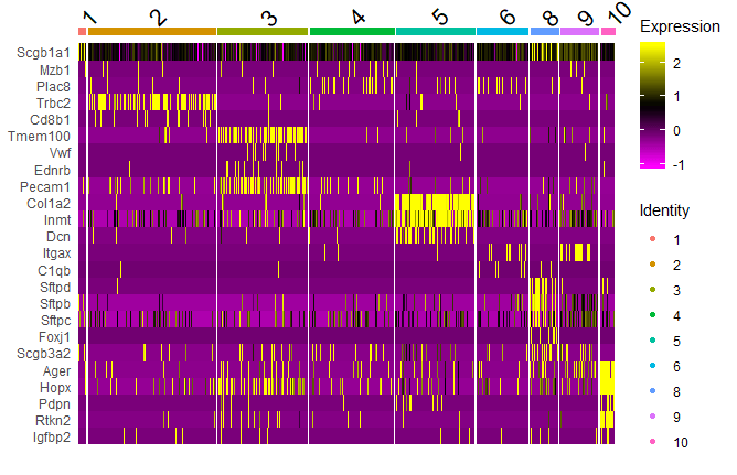
Heat map
DoHeatmap(object = seuratobj, features = features)
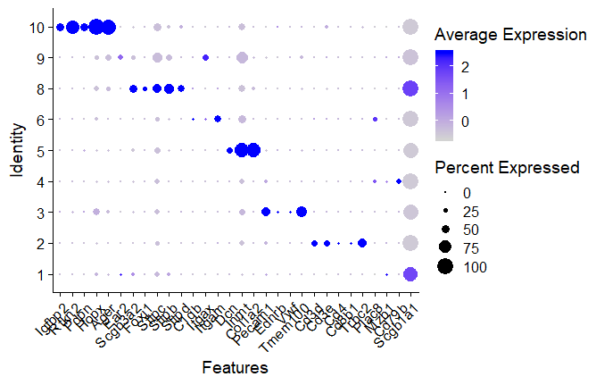
DotPlot
DotPlot(seuratobj, features = features) + RotatedAxis()
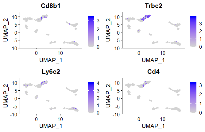
Feature plots
Highlight marker gene expression in dimension reduction plot such as UMAP or tSNE.
To reduce computing time we only select a few features
#selected marker genes for cell type
features <- c("Cd8b1","Trbc2","Ly6c2","Cd4")
#UMAP feature plot colour coded by defined feature
FeaturePlot(seuratobj, features = features,reduction = "umap")
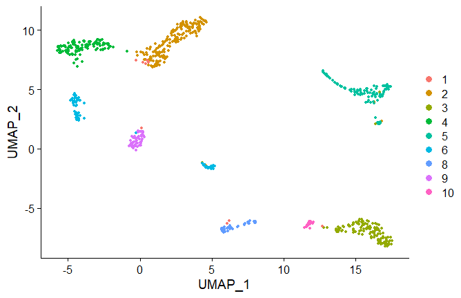
Step 7: Dimension reduction plots
The goal of dimension reduction plots is to visualize single cell data by placing similar cells in close proximity in a low-dimensional space. Seurat offers non-linear dimension reduction techniques such as UMAP and tSNE.
PCA
seuratobj <- RunPCA(seuratobj, features = VariableFeatures(object = seuratobj)) DimPlot(seuratobj, reduction = “pca”) ElbowPlot(seuratobj) #to determine the dimensionality of the datasetUMAP
seuratobj <- RunPCA(seuratobj, features = VariableFeatures(object = seuratobj)) DimPlot(seuratobj, reduction = “pca”) ElbowPlot(seuratobj) #to determine the dimensionality of the dataset
If you haven’t installed UMAP, type reticulate::py_install(packages=’umap-’learn’)
seuratobj <- RunUMAP(seuratobj, dims = 1:10)
DimPlot(seuratobj, dims=c(1,2), reduction = "umap",label=TRUE)
SaveRDS(seuratobj, file=”../output/filename.rds”)
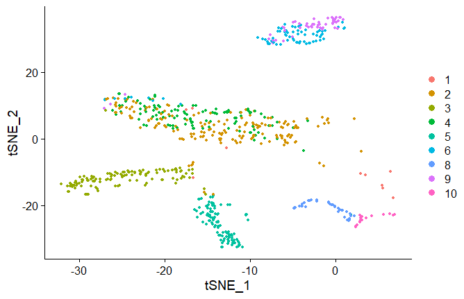
tSNE
#similar to the PCA and UMAP method, run RunTSNE
seuratobj <- RunTSNE(seuratobj)
DimPlot(seuratobj, reduction = "tsne")
Many more visualization option for your data can be found under vignettes on the Satija lab website.
This vignette is very useful if you are trying to compare two conditions.
We hope this tutorial was useful to you and that it will enable to you to take data into your own hands. Should you have any questions you can contact us here .
